Documentation -
Tutorial -
Sample Cuts
FuzzyFilter - Tutorial
The FuzzyFilter allows the definition of FuzzyCuts that (can) surpass classical cuts when more than two observables are involved.
Furthermore, the information of observables with heavily overlapping background and interesting data can be used in fuzzy analysis.
This quickstart tutorial gives a short introduction on how to use the FuzzyFilter Hardcallback.
I. General
- FuzzyFilter generates the following subevents:
- FUZZY_RATING[0]:
- 1 - event passed the FuzzyFilter
- 0 - event is marked as 'bad event' (background)
- FUZZY_WEIGHT[0]:
- corresponds to X (see FuzzyFilter Documentation)
- FUZZY_WEIGHT[1]:
- corresponds to Y (see FuzzyFilter Documentation)
- FuzzyFilter has the following BrokerVariables:
- refHistoFile:
- hbook-file that contains the reference histograms
- actualFuzzyCut:
- can be used to load FuzzyCuts from hoc-files, e.g. broker("FuzzyFilter:actualFuzzyCut", "s13atomic.ff");
- energyRange:
- determines the energy range
covered by min/mid/max. The range from
minRampEnergy to maxRampEnergy is divided into three
sections and energyRange percent of each range is
used to create the (energy) projections of all histograms in
FuzzyFilter (default: energyRange = 33)
- minRampEnergy:
- lower limit for the beam energy
- maxRampEnergy:
- upper limit for the beam energy
minRampEnergy and maxRampEnergy must be set properly,
also for flattop data.
- Use the new menu item FUZZY in the YODA menubar to raise/hide the FuzzyFilter GUI (Graphical User Interface)
- Whenever FuzzyFilter is enabled, FUZZY.hoc is loaded. It is highly recommended not to touch/edit this SoftCallback.
II. How to make your own FuzzyCut
EXAMPLE: Generation of a FuzzyCut to seperate elastic and background events for CH2-data.
General remarks are printed in normal font, instructions for the generation of the sample cut are printed in italic font .
You will need a SoftCallback (hoc-file) in order to monitor the success of your actions.
Write your own one or use/modify this one.
You have to assign appropriate values to the broker variables
minRampEnergy and maxRampEnergy. For flattop data
minRampEnergy and maxRampEnergy have the same value and
the energy states 'mid' and 'high' will be ignored (see documentation (13)
for further details).
STEP 1: Generation of reference histograms
Reference histograms are distributions of the elastic content of the data.
Since the aim of analysis is to seperate the elastic content from the background, it might seem paradoxical to start the analysis with what you hope to get at the end of the analyzing process.
Usually one has some ideas on how to supress huge amounts of background and only the small remaining part that passes these conditions causes real headache.
The condition 'kinematic deficit < 8' selects almost all elastic events and eliminates a major part of the background but to get rid off the non-elastic events with a kinematic deficit below 8 deserves more sophisticated tactics.
The FuzzyFilter needs raw estimates of how the elastic content looks like.
These estimates are the reference histograms and they are used in the further analysis to model memberfunctions.
For CH2-data it is obvious that carbon-subtracted data is the best reference one can supply.
Always use (and modify) refHistos2d.hoc to generate the refHisto.hbook-files but do not change the histogram definitions.
You can now make your own reference histogramms or use this one (for use with beamtime nov'97(13) exp3-data).
Right-click and select 'save link as..' to download the hbook-file.
Use the 'load ref.' Button from the FuzzyFilter GUI or the broker-variable 'refHistoFile' to load new reference data.
Step 2: Observable selection
The FuzzyFilter combines the information of several observables and generates one (or two) new observable(s).
This reduction of dimensionaltity allows to use the information of many observables at the same time, i.e. 'parallel', whereas in the classical analysis the cuts are applied sequentially.
The latter corresponds to operations on linear projections of the high-dimensional vectorspace spanned by the observables.
Event classes that are seperated in the high dimensional observable-space but overlapp in all linear projections can not be seperated with sequential cuts.
The FuzzyFilter generates a 1- or 2-dimensional non-linear projection of the observable
space.
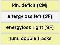 Choose observables by using the 'add' button in the 'Observable' part of the FuzzyFilter GUI.
The 'delete' button deletes the highlighted observable from the observable list.
For the CH2-Cut, ALPHA[0] (kin. deficit), FIRST_MATCH[10] (energyloss left SF), FIRST_MATCH[11] (energyloss right SF) and VERTEX_FT[5] (number of double tracks) might be interesting.
Press the 'update' button to bring YODA up to date (this generates and reloads FUZZY.hoc).
Step 3: Memberfunctions
Memberfunctions are the heart of the FuzzyFilter.
They reflect the actual knowledge about the data by judging the quality of every single event.
Each observable has its own memberfunction and it is the value of the memberfunction (and not the value of the subevent) that is used in the further fuzzy analysis.
You can think of memberfunctions as probability distributions that tell you with what probability a single value of an observable corresponds to an elastic event.
The memberfunction for the kinematic deficit has values near 1 for small alpha but decreases fast with increasing values of alpha since the probability that the corresponding event was an elastic one also decreases with higher alpha.
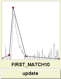 For an infinite amount of data (perfect statistic) the memberfunction is the same as
(distribution for the elastic content)/(distribution for complete data).
In our CH2-example, the complete data is the CH2-data and the elastic content is the carbon-subtracted data.
Start YODA to accumulate some CH2-data.
You can plot both histograms or their quotient (which is the best estimate for the memberfunction) in the memberfunction window by pressing the appropriate buttons in the Histogram section of the FuzzyFilter GUI.
The histograms are updated every time a button is pressed.
Now press the different observable buttons in your observable list and model the memberfunction (the black line in the meberfunction window) after the 'member' histogram.
The documentation explains the commands.
It is not necessary to model each detail of the member histogram, a rough fit with
two to six linear segments works well.
Keep in mind, that the quality of the member histogram depends on the quality of the reference data.
Do not forget to press the 'update' button to bring YODA up to date (memberfunctions are transfered).
Step 4: Fuzzy operator
The further processing of the memberfunctions is defined in the Fuzzy Operator section.
Here, one can choose which observables should be combined to build the new observables 'X' or 'Y', respectively.
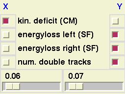 The sliders at the bottom set the values for the gamma-parameter of the 'X' or the 'Y' combination, respectively (see documentation).
Mark the kinematic deficit for the 'X' combination and the remaining three observables for the 'Y' combination.
Set the 'Y' gamma slider to a value around 0.4.
Any changes in this section (sliders, checkbuttons) affect YODA in realtime (no need to press any update-buttons).
Nevertheless, it is advisable to press YODA's 'Clear Histograms' button after changes, since this does also clear the 'X', 'Y' and 'X vs. Y' plots.
Step 5: FuzzyCuts
A FuzzyCut is a cut on the new observables 'X' and/or 'Y'.
The 1d-Cut window allows the definition of a one-dimensional cut.
This is useful when only few observables are combined to a single new observable.
Refer to the documentation for the commands.
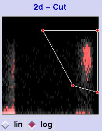 A two-dimensional cut can be plotted in the 2d-Cut window.
Since the values of the memberfunctions reflect the probability that a single event is elastic (in general: interesting), the good events are mapped to the top right corner of the histogram whereas the background is mapped to the lower left corner.
Events that are good in one observable but bad at the other are mapped to the top left or bottom right corner, respectively.
It is a matter of experience to find the optimal polygon but keep in mind that 'top right is always good'.
Start YODA and press the 'log' button to bring up the 2-dimensional histogram.
Press 'log' again to update the plot.
You can use the zoom-commands to optimize the view.
Press the middle mouse button to bring up a three-segmented polygon and use the mouse to modify it (-->documentation).
A four-segmented polygon like the one in the picture is a good starting point.
Do not forget to press the 'log' button in order to transfer the new polygon coordinates to YODA (red circles: YODA is up to date)
Now you can use the new subevent FUZZY_RATING[0] to select the good events in your further analysis.
 Choose observables by using the 'add' button in the 'Observable' part of the FuzzyFilter GUI.
The 'delete' button deletes the highlighted observable from the observable list.
 For an infinite amount of data (perfect statistic) the memberfunction is the same as
 The sliders at the bottom set the values for the gamma-parameter of the 'X' or the 'Y' combination, respectively (see documentation).
 A two-dimensional cut can be plotted in the 2d-Cut window.
Since the values of the memberfunctions reflect the probability that a single event is elastic (in general: interesting), the good events are mapped to the top right corner of the histogram whereas the background is mapped to the lower left corner.
Events that are good in one observable but bad at the other are mapped to the top left or bottom right corner, respectively.
It is a matter of experience to find the optimal polygon but keep in mind that 'top right is always good'.